Sims.jl
A Julia package for equation-based modeling and simulations.
Background
Sims is like a lite version of Modelica. This package is for non-causal modeling in Julia. The idea behind non-causal modeling is that the user develops models based on components which are described by a set of equations. A tool can then transform the equations and solve the differential algebraic equations. Non-causal models tend to match their physical counterparts in terms of their specification and implementation.
Causal modeling is where all signals have an input and an output, and the flow of information is clear. Simulink is the highest-profile example. The problem with causal modeling is that it is difficult to build up models from components.
The highest profile noncausal modeling tools are in the Modelica family. The MathWorks company also has Simscape that uses Matlab notation. Modelica is an object-oriented, open language with multiple implementations. It is a large, complex, powerful language with an extensive standard library of components.
This implementation follows the work of David Broman (thesis and code) and George Giorgidze (Hydra code and thesis) and Henrik Nilsson and their functional hybrid modeling. Sims is most similar to Modelyze by David Broman (report).
Two solvers are available to solve the implicit DAE's generated. The default is DASKR, a derivative of DASSL with root finding. A solver based on the Sundials package is also available.
Installation
Sims is an installable package. To install Sims, use the following:
Pkg.add("Sims")
Sims.jl has one main module named Sims and the following submodules:
-
Sims.Lib-- the standard library -
Sims.Examples-- example models, including: Sims.Examples.BasicsSims.Examples.LibSims.Examples.Neural
Basic example
Sims defines a basic symbolic class used for unknown variables in the model. As unknown variables are evaluated, expressions (of type MExpr) are built up.
julia> using Sims

julia> a = Unknown()
##1243

julia> a * (a + 1)
MExpr(*(##1243,+(##1243,1)))
In a simulation, the unknowns are to be solved based on a set of equations. Equations are built from device models.
A device model is a function that returns a vector of equations or other devices that also return lists of equations. The equations each are assumed equal to zero. So,
der(y) = x + 1
Should be entered as:
der(y) - (x+1)
der indicates a derivative.
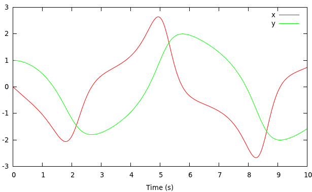
The Van Der Pol oscillator is a simple problem with two equations and two unknowns:
function Vanderpol()
    y = Unknown(1.0, "y")   # The 1.0 is the initial value. "y" is for plotting.
    x = Unknown("x")        # The initial value is zero if not given.
    # The following gives the return value which is a list of equations.
    # Expressions with Unknowns are kept as expressions. Expressions of
    # regular variables are evaluated immediately.
    Equation[
        # The -1.0 in der(x, -1.0) is the initial value for the derivative
        der(x, -1.0) - ((1 - y^2) * x - y)      # == 0 is assumed
        der(y) - x
    ]
end

y = sim(Vanderpol(), 10.0) # Run the simulation to 10 seconds and return
                           # the result as an array.
# plot the results with Winston
using Winston
wplot(y)
Here are the results:

An @equations macro is provided to return Equation[] allowing for
the use of equals in equations, so the example above can be:
function Vanderpol()
    y = Unknown(1.0, "y")
    x = Unknown("x")
    @equations begin
        der(x, -1.0) = (1 - y^2) * x - y
        der(y) = x
    end
end

y = sim(Vanderpol(), 10.0) # Run the simulation to 10 seconds and return
                           # the result as an array.
# plot the results with Winston
wplot(y)
Electrical example
This example shows definitions of several electrical components. Each is again a function that returns a list of equations. Equations are expressions (type MExpr) that includes other expressions and unknowns (type Unknown).
Arguments to each function are model parameters. These normally include nodes specifying connectivity followed by parameters specifying model characteristics.
Models can contain models or other functions that return equations. The function Branch is a special function that returns an equation specifying relationships between nodes and flows. It also acts as an indicator to mark nodes. In the flattening/elaboration process, equations are created to sum flows (in this case electrical currents) to zero at all nodes. RefBranch is another special function for marking nodes and flow variables.
Nodes passed as parameters or created with ElectricalNode() are simply unknowns. For these electrical examples, a node is simply an unknown voltage.
function Resistor(n1, n2, R::Real)
    i = Current()   # This is simply an Unknown.
    v = Voltage()
    @equations begin
        Branch(n1, n2, v, i)
        R * i = v
    end
end

function Capacitor(n1, n2, C::Real)
    i = Current()
    v = Voltage()
    @equations begin
        Branch(n1, n2, v, i)
        C * der(v) = i
    end
end
What follows is a top-level circuit definition. In this case, there are no input parameters. The ground reference "g" is assigned zero volts.
All of the equations returned in the list of equations are other models with various parameters.
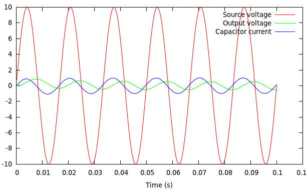
function Circuit()
    n1 = Voltage("Source voltage")   # The string indicates labeling for plots
    n2 = Voltage("Output voltage")
    n3 = Voltage()
    g = 0.0  # A ground has zero volts; it's not an unknown.
    Equation[
        SineVoltage(n1, g, 10.0, 60.0)
        Resistor(n1, n2, 10.0)
        Resistor(n2, g, 5.0)
        SeriesProbe(n2, n3, "Capacitor current")
        Capacitor(n3, g, 5.0e-3)
    ]
end

ckt = Circuit()
ckt_y = sim(ckt, 0.1)
gplot(ckt_y)
Here are the results:

Initialization and Solving Sets of Equations
Sims initialization is still weak, but it is developed enough to be
able to solve non-differential equations. Here is a small example
where two Unknowns, x and y, are solved based on the following two
equations:
function test()
    @unknown x y
    @equations begin
        2*x - y   = exp(-x)
         -x + 2*y = exp(-y)
    end
end

solution = solve(create_sim(test()))
Hybrid Modeling and Structural Variability
Sims supports basic hybrid modeling, including the ability to handle structural model changes. Consider the following example:
This model starts as a pendulum, then the wire breaks, and the ball goes into free fall. Sims handles this much like Hydra; the model is recompiled. Because Julia can compile code just-in-time (JIT), this happens relatively quickly. After the pendulum breaks, the ball bounces around in a box. This shows off another feature of Sims: handling nonstructural events. Each time the wall is hit, the velocity is adjusted for the "bounce".
Here is an animation of the results. Note that the actual animation was done in R, not Julia.
